Portfolio Rebalancing and Spend Rule Analysis
This page contains a project I worked on as part of a University assignment. The project was for a subject called “Portfolio Theory and Management” and the aim was to provide a fund with a diverse portfolio, earning a target of 5.5% real return per annum. The fund would also like to make real donations of 5% per annum.
The lecturer loved that I used python to code up more portfolio samples, it’s definitely not a typical thing to do!
We created a Risk Parity portfolio, as well as a portfolio created by the solver function in excel. My part of the group assignment was to stress test both portfolios.
A risk parity portfolio is created by each asset having a weight such that it’s risk is equal to all other assets. That is, each asset contributes an equal amount of risk to the portfolio.
In my extension of this, I wrote some code to analyse different spend rules and rebalancing methods.
The portfolio’s consisted of 5 different asset types. I created a Monte Carlo simulation for each of these, and simulated the portfolio, using the asset weights calculated from both the Risk Parity and Solver Portfolios.
The following charts show the difference between Range and Quarterly rebalancing on spend completion rates. The range for a rebalance was 10%. This means that when an asset has weight in a portfolio above or below 10% of its initial weighting, a rebalance occurs, re-weighting all the assets. For example, if equities make up 30% of the portfolio initially, when the equities grow in such a way as to make up 40% of the portfolio, a rebalance would occur. This range rebalancing is different to quarterly rebalancing. In quarterly rebalancing, the portfolio is rebalanced at the end of every quarter.
The spending rule, as stated earlier, is that the fund wants to spend 5% per year, but the key part is they can only do so if the portfolio value is above the initial value. This enables the fund to recuperate losses much better and allows them to spend more in the future.
As part of my simulations, I created some charts to show some useful information
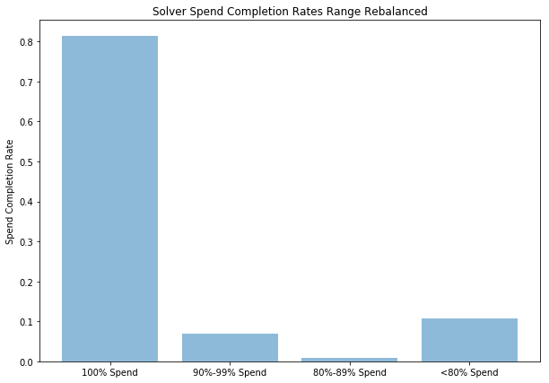
Solver Portfolio: Spend Completion Rates using Range Rebalancing
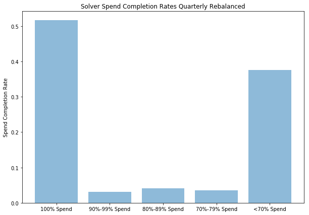
Solver Portfolio: Spend Completion Rates using Quarterly Rebalancing
As you can see from these figures, the range rebalanced portfolio allows much more consistent levels of spending.
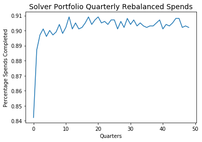
Spending Rates for Range Rebalanced Portfolio
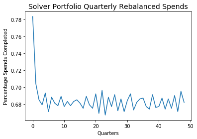
Spending Rates for Quarterly Rebalanced Portfolio
The first figure title should be “Range Rebalanced Spends”. The same situation again unfolds, that the range rebalancing portfolio allows a spending completion rate much higher than the quarterly rebalanced portfolio.
The rate is not 100% as some portfolios drop below the initial real value of the portfolio and hence can’t complete the spend.
Another aspect to analyse in the rebalancing rates. This is important to compare the two portfolio’s and see how often any asset goes outside the allowed range.
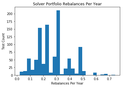
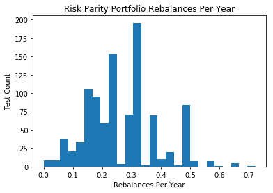
As can be seen in these images, the rebalancing is roughly the same per year, at around 0.25-0.3 rebalances per year. Tighter ranges would mean more rebalances per year.
Further analysis could include possible modifications to the spend rule to maximise spend completion rates, and optimal rebalancing ranges to maximise portfolio value.
If you’d like to read my code, please email me at [email protected] .